Customer Segmentation
I used K-Means to group 200 mall customers by age, gender, income, and spending score, then compared the groups to see where different marketing tests might make sense.
Overview
The question
The dataset is small: 200 customers, with age, gender, annual income, and a mall-assigned Spending Score from 1 to 100.
I used it to explore a straightforward segmentation question:
Can those variables separate customers into groups that are different enough to justify testing different marketing approaches?
Income alone did not answer much. Customers at similar income levels could have very different spending scores, and customers with different incomes could show similar spending behavior.
That made the relationship between the variables more useful than any one variable by itself.
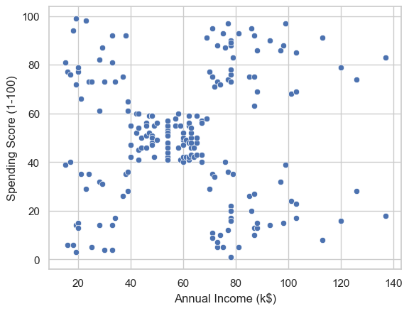
Income versus spending score, all 200 customers. At similar income levels, spending scores run from 1 to 99.
The project eventually moved from simple one-variable clustering to a final model using age, encoded gender, annual income, and spending score together. Before fitting that model, I standardized the features so a variable with larger raw values, such as income, would not dominate the distance calculation.
Starting with the simpler view
Before adding all four variables, I looked at income and spending score together.
That two-dimensional view made one thing easy to see: income did not map neatly to spending behavior.
There were high-income customers with high spending scores and high-income customers with very low scores. The same split appeared at lower income levels.
A five-cluster bivariate model made those differences easier to inspect, but I did not stop there. Age and gender were still missing from the grouping, so I treated the income-versus-spending model as a baseline rather than the final segmentation.
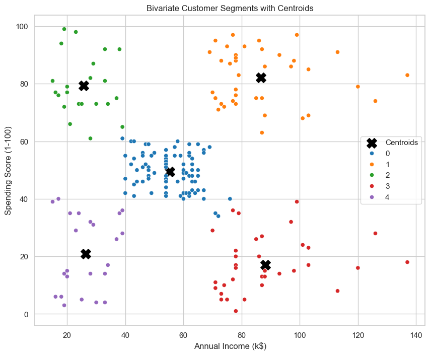
The income + spending score baseline: five clusters and their centroids. Age and gender are not part of this model.
Building the final model
For the final clustering pass, I used four inputs:
- Age
- Annual Income
- Spending Score
- encoded Gender
Gender was converted into a numeric dummy variable, then all four inputs were standardized with StandardScaler.
I ran K-Means across different values of K and used the multivariate elbow curve to choose five clusters for the final model.
I describe that as a practical modeling choice, not proof that five permanent customer types exist. K-Means will partition the data it receives, and this sample is too small to claim that the same five groups would necessarily appear in another customer base.
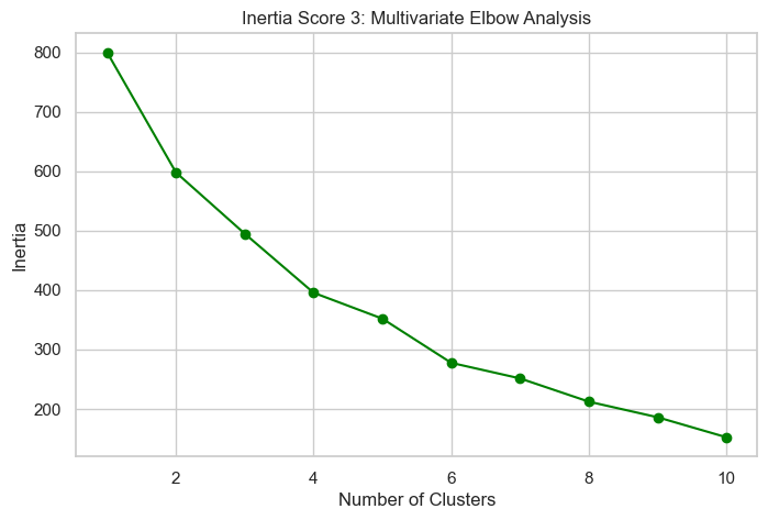
The multivariate elbow curve. I read the bend around five clusters as a practical model choice for this sample, not proof that exactly five customer types exist.
What the five groups looked like
The final model created five groups with noticeably different average profiles. The labels below describe what is actually in the data rather than turning each cluster into a marketing stereotype.
- Cluster 2 Younger · mid-income · highest spending scoreCustomers 42Avg age 28.7Avg income $60.9KAvg spending score70.2
- Cluster 4 Younger · lower-income · mid-high spending scoreCustomers 38Avg age 27.3Avg income $38.8KAvg spending score56.2
- Cluster 3 Higher-income · mid-range spending scoreCustomers 49Avg age 37.9Avg income $82.1KAvg spending score54.4
- Cluster 0 Older · moderate-income · lower spending scoreCustomers 51Avg age 56.5Avg income $46.1KAvg spending score39.3
- Cluster 1 Higher-income · lowest spending scoreCustomers 20Avg age 39.5Avg income $85.2KAvg spending score14.1
Cluster averages from the final four-variable model · score bars use the score's full 1 to 100 index range
One metric I would describe differently now
Spending Score ÷ Annual Income = exploratory score-to-income index
During the analysis, I also created a Spend_Income_Ratio by dividing Spending Score by annual income. It helped me compare profiles during exploration, and Cluster 4 had the highest average value at 1.85.
But Spending Score is an index from 1 to 100, not an amount of money spent. I would not describe 1.85 as the share of a customer's income going to the mall, or use it as proof that one group is more financially "efficient" than another.
I would describe it for what it is: a derived score-to-income index that helped me notice customers whose spending score was relatively high compared with their reported income. The calculation is useful for exploration, but the interpretation has to stay within what the variables actually measure.
What stood out
The most useful contrast was at the high-income end.
Cluster 3 averaged about $82.1K in annual income with a spending score of 54.4. Cluster 1 averaged slightly more income, about $85.2K, but its average spending score was only 14.1.
Score bars use the score's full 1 to 100 index range
The income difference between those groups is small compared with the difference in their spending scores.
That is the kind of contrast segmentation is useful for: it gives me two groups that look similar on one dimension but behave very differently on another.
What the data does not tell me is why.
The low score could reflect product mix, visit frequency, customer preferences, the way the Spending Score was constructed, or something else entirely. This dataset does not contain enough information to choose between those explanations.
What I would test next
I would use these segments as starting points for experiments, not as finished customer personas.
Cluster 2 is the clearest first group to test because it has the highest average spending score in the sample.
Cluster 1 is interesting for the opposite reason: relatively high income paired with the lowest average spending score.
Rather than assuming what either group wants, I would test different messages or offers and measure an actual outcome such as conversion, visit frequency, basket value, or response rate.
That would answer the question this dataset cannot:
Do these clusters actually help predict who responds differently?
If they do, the segmentation becomes useful beyond describing the sample. If they do not, I would change the features or the segmentation rather than forcing a marketing story onto the clusters.
How I built it
I worked through the project in stages instead of jumping directly to the final K-Means model.
I started with exploratory analysis of the individual variables, then looked at relationships between income, spending score, age, and gender. From there I built:
- Income-only clustering
- A simple baseline for understanding how K-Means grouped one variable.
- Income + Spending Score clustering
- A two-dimensional model that exposed customers with similar incomes but very different spending scores.
- Four-variable clustering
- The final model using age, encoded gender, income, and spending score after standardization.
I used the elbow method at each stage to inspect how the cluster structure changed as more information entered the model.
The final output includes the original customer records, their earlier clustering labels, and the final multivariate cluster assignment.
The GitHub repository contains the full notebook, all 16 visualizations, and the final labeled customer dataset.
Reflection
This project was useful because it was one of my first attempts to move beyond descriptive charts and let an algorithm create groups from several variables at once.
The part I would approach more carefully now is the interpretation.
It is easy to run K-Means, give every cluster a memorable name, and immediately attach a marketing campaign to it. The harder question is whether the source data actually supports that story.
Here, the clustering gives me five different profiles in this 200-customer sample. It does not give me customer lifetime value, campaign response, profit, product preference, or the reason someone has a particular spending score.
If I continued the project, I would validate the clusters on a larger dataset, compare more than one clustering-quality measure, and connect the segments to a real behavioral outcome before treating them as a marketing strategy.
That is the part of the project I find more useful now: not just getting K-Means to run, but getting clearer about the difference between a cluster the model creates and a customer segment a business can actually act on.